Gradient Boosting for Regression
This post is basically based on A Gentle Introduction to Gradient Boosting - Cheng Li.
What is Gradient Boosting
In each stage, a weak learner is introduced to compensate the shortcomings of existing weak learners.
In Gradient Boosting, “shortcomings” are identified by gradients.
Recall that, in Adaboost, “shortcomings” are identified by high-weight data points.
Both high-weight data points and gradients tell us how to improve our model.
How to understand Gradient Boosting
I found an example from A Gentle Introduction to Gradient Boosting - Cheng Li quite straightforward and I will borrow it here.
Additional model \(h\)
Suppose you are playing a game. You are given \((x_1, y_1),(x_2, y_2), ...,(x_n, y_n)\), and the task is to fit a model \(F(x)\) to minimize square loss.
Suppose your friend wants to help you and gives you a model \(F\). You check his model and find the model is good but not perfect.
There are some mistakes: \(F(x_1) = 0.8\), while \(y_1 = 0.9\), and \(F(x_2) = 1.4\) while \(y_2 = 1.3\)… How can you improve this model?
A simple solution is to fit an additional regression model \(h(x)\) so that
\[F(x_1)+h(x_1) = y_1\] \[F(x_2)+h(x_2) = y_2\] \[...\] \[F(x_n)+h(x_n) = y_2\]That is, we want to fit a regression model \(h(x)\) to the data
\[(x_1, y_1-F(x_1)),(x_2, y_2-F(x_2)), ...,(x_n, y_n-F(x_n))\]Here \(y_i-F(x_i)\) is called residuals. These are the parts that existing model \(F\) cannot do well. The role of \(h\) is to compensate the shortcoming of existing model \(F\).
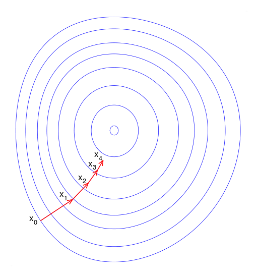
Gradient Descent
Gradient descent is a numerical way to minimize the function towards the negetive gradient direction.
\[\theta _i := \theta _i - \rho \frac{\partial J}{\partial \theta _i}\]
If we choose the squared error as loss function:
\[L(y,F(x))=\frac{1}{2}(y-F(x))^2\]and we want to minimize
\[J = \sum _i L(y_i,F(x_i))\]If we look \(F(x_i)\) as variables and take derivatives
\[\frac{\partial J}{\partial F(x_i)} = \frac{\partial \sum _i L(y_i,F(x_i))}{\partial F(x_i)} = \frac{\partial L(y_i,F(x_i))}{\partial F(x_i)} = F(x_i) - y_i\]Hence residuals can be interpreted as negative gradients:
\[y_i - F(x_i) = - \frac{\partial J}{\partial F(x_i)}\]Gradient Boosting
In boosting, we update \(F(x)\) with additional \(h(x)\), that is
\[\begin{align} F(x_i) &:= F(x_i) + h(x_i) \\ F(x_i) &:= F(x_i) + y_i - F(x_i) \\ F(x_i) &:= F(x_i) - 1\frac{\partial J}{\partial F(x_i)} \\ \theta _i &:= \theta _i - \rho \frac{\partial J}{\partial \theta _i} \end{align}\]that is, we are using the following equivalence relation:
\[\begin{align} \text{residual} &\Leftrightarrow \text{negative gradient} \\ \text{fit } h \text{ to residual} &\Leftrightarrow \text{fit } h \text{ to negative gradient} \\ \text{update } F \text{ based on residual} &\Leftrightarrow \text{update } F \text{ based on negative gradient} \end{align}\]Now we have an algorithm of gradient boosting for regression:
Start with an initial model \(F(x)\) Iterate until converge:
- Calculate negetive gradients \(-g(x_i) = \frac{\partial L(y_i,F(x_i))}{\partial F(x_i)}\)
- Fit a regression model \(h\) to negetive gradients \(-g(x_i)\)
- \(F := F + \rho h\) where \(\rho = 1\)
The benefit of formulating this algorithm using gradients is that it allows us to consider other loss functions and derive the corresponding algorithms in the same way.
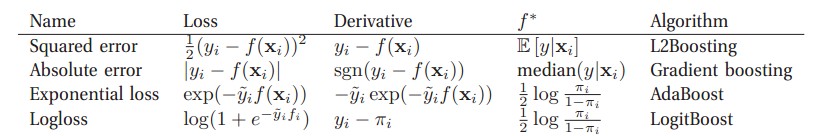
One reason to consider other loss functions instead of squared loss is that it’s not robust to outliers. Other loss functions, such as absolute loss and Huber loss are more robust to outliers.
A summary of different loss functions and related boosting can be found in Machine Learning - A Probabilistic Perspective - Kevin P. Murphy