Clustering
This post is based on the content from Lecture 6: Partitioning Data into Clusters, Finding Categories in Data - Cosma Shalizi
As we might have know, clustering is to categorize the samples into some parts while we do not know the labels initially. Learning problems can be divided into three categories as follows:
| Known classes? | Class labels | Type of learning problem |
|---|---|---|
| Yes | Given for training data | Classification; supervised learning |
| Yes | Hints/feedback | Semi-supervised learning |
| No | None | Clustering; unsupervised learning |
An interesting comment from Cosma Shalizi is that “The point being, even when you have what you are told is a supervised learning problem with labeled data, it can be worth treating it as unsupervised learning problem.” He has some very impressive reasons for doing so.
The $k$-means algorithm
A simple frame of the \(k\)-means algorithm is shown as follows:
- Guess the number of clusters, \(k\)
- Guess the location of cluster means
- Assign each point to the nearest mean
- Re-compute the mean for each cluster
- If the means are unchanged, exit; otherwise go back to (3)
The objective function for \(k\)-means is the sum-of-squares for the clusters:
\[SS \equiv \sum_C \sum_{i\in C} \parallel x_i - m_C\parallel ^2\] \[m_C \equiv \frac{1}{n_C} \sum_{i \in C} x_i\]\(m_C\) is the mean for cluster \(C\), and \(n_C\) is the number of points in that cluster.
The within-cluster variance for cluster \(C\) is
\[V_C \equiv \frac{1}{n_C} \sum_{i\in C} \parallel x_i - m_C\parallel ^2\]so
\[SS \equiv \sum_C n_C V_C\]That is, \(k\)-means want to minimize the within-cluster variance times the cluster size, summed over clusters. Each step of \(k\)-means reduces the sum-of-squares. The sum-of-squares is always positive. Therefore \(k\)-means must eventually stop, no matter where it was started. However, it may not stop at the best solution. That is, \(k\)-means is a local search algorithm.
Hierarchical clustering
As its name suggests, instead of giving a flat partition as \(k\)-means, hierarchical clustering can give us a more organized ourput like a tree.
Ward’s method
Ward’s method is another algorithm for finding a partition with small sum of squares. Instead of starting with a large sum of squares and reducing it, you start with a small sum of squares (by using lots of clusters) and then increasing it.
A simple frame of Ward’s method is shown as follows:
- Start with each point in a cluster by itself (sum of squares = 0).
- Merge two clusters, in order to produce the smallest increase in the sum of squares (the smallest merging cost).
- Keep merging until you’ve reached \(k\) clusters.
The merging cost is the increase in sum of squares when you merge two clusters (\(A\) and \(B\), say), and has a simple formula:
\[\begin{align} \Delta(A,B) &= \sum_{i\in A \cup B} \parallel x_i - m_{A \cup B} \parallel ^2 - \sum_{i\in A} \parallel x_i - m_A\parallel ^2 - \sum_{i\in B} \parallel x_i - m_B\parallel ^2 \\ &= \frac{n_A n_B}{n_A + n_B} \parallel m_A - m_B \parallel ^2 \end{align}\]Single-link algorithm
A simple frame of single-link method is shown as follows:
- Start with each point in a cluster by itself (sum of squares = 0).
- Merge the two clusters with smallest gap (distance between the two closest points)
- Keep merging until you’ve reached \(k\) clusters.
It’s called “single link” because it will merge clusters so long as any two points in them are close (i.e., there is one link). This algorithm only wants separation, and doesn’t care about compactness or balance, which can lead to new problems.
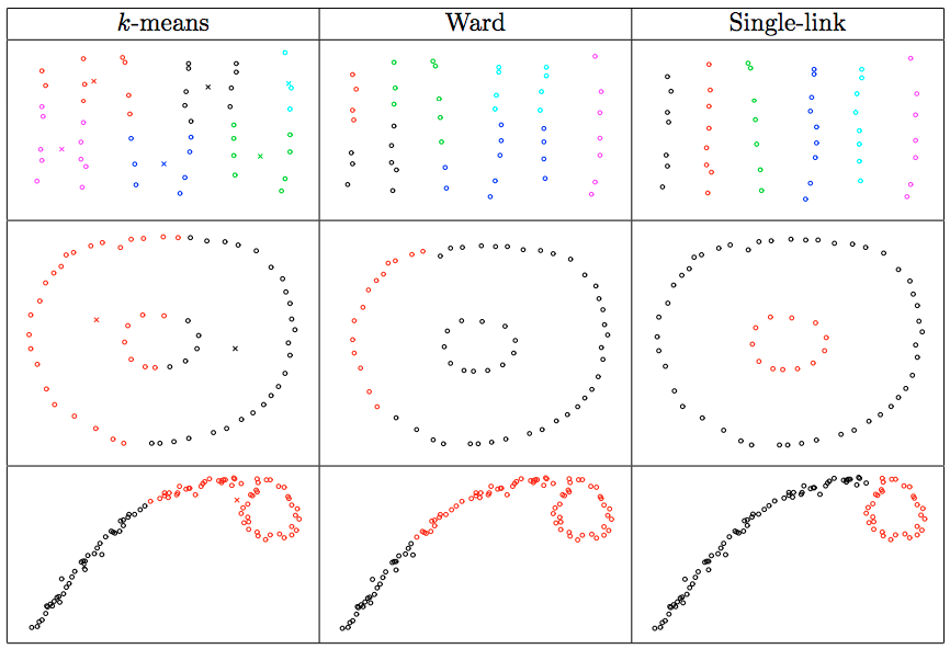
The following are some cases where single-link method outperforms \(k\)-means and Ward’s method. (Figure comes from Lecture 6: Partitioning Data into Clusters, Finding Categories in Data - Cosma Shalizi).
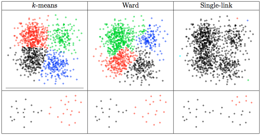
The following are some cases where single-link method is worse than \(k\)-means and Ward’s method. (Figure comes from Lecture 6: Partitioning Data into Clusters, Finding Categories in Data - Cosma Shalizi).